This section sets out the method followed to identify the relevant indicators and process the data to generate the maps that comprise this study. This method is designed to be easily replicated.

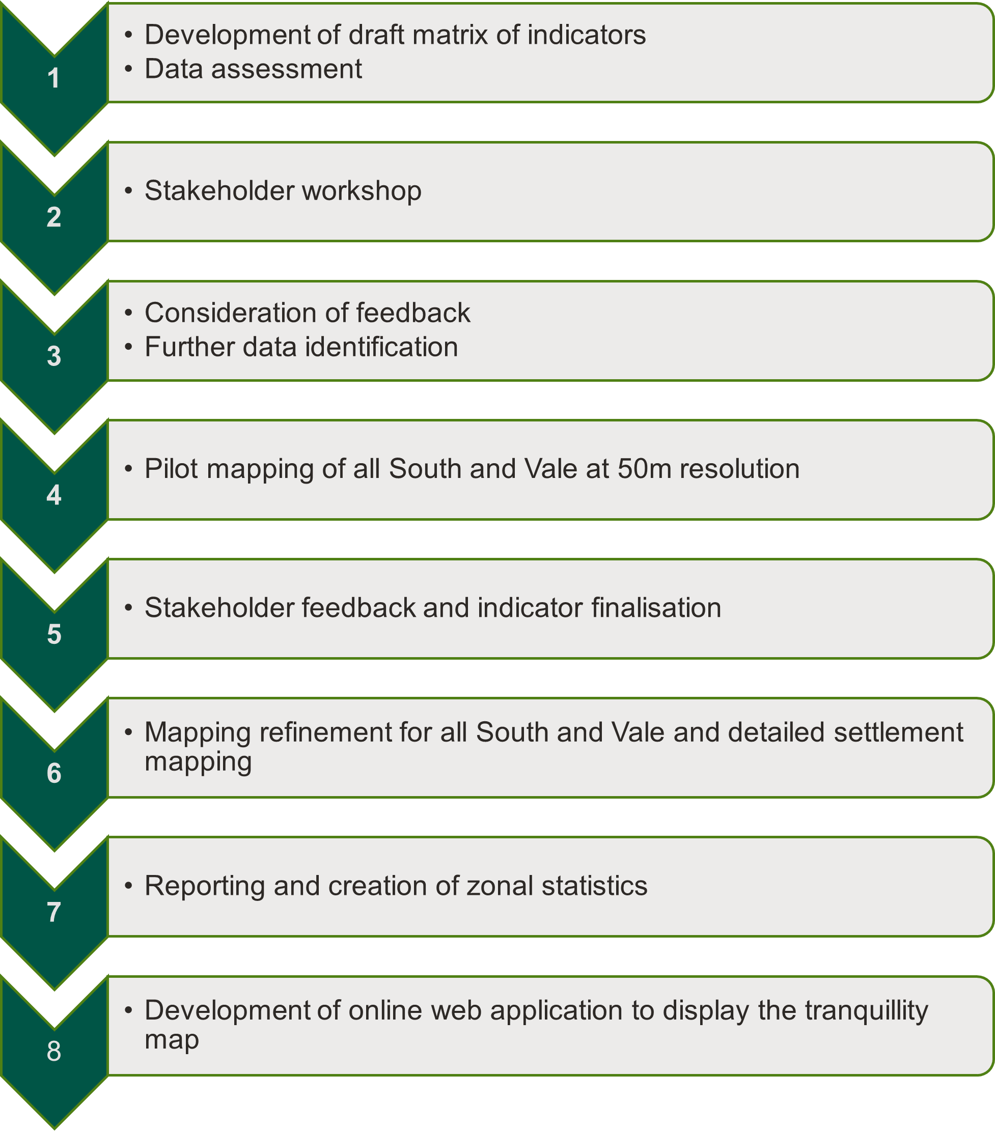
The approach taken to develop the mapping methodology followed the stages set out in Figure ‎2.1.

Figure 2.1: Summary of approach

The methodology for this study is based on the Tranquillity Mapping: Developing a Robust Methodology for Planning Support Technical Report produced by Northumbria University for CPRE in 2008 [See reference [i]]. It also draws on the experience in assessing and mapping tranquillity which LUC has built up in past projects, such as Tranquillity and Place in Wales [See reference [ii]] and Tranquillity Mapping for Central Bedfordshire Council [See reference [iii]].

[i] Northumbria University for CPRE. (2008). Tranquillity Mapping: Developing a Robust Methodology for Planning Support Technical Report. Available at: https://www.cpre.org.uk/resources/tranquillity-mapping-developing-a-robust-methodology-for-planning-support/

[ii] Green C, Manson D, Chamberlain K. (2022). NRW Report No: 569, 185 pp, NRW. Available at: https://storymaps.arcgis.com/stories/865c1876d9f64280a3dfc6e2769a46a5

[iii] LUC. (2022). Central Bedfordshire Tranquillity Strategy: Supporting the Assessment of Relative Tranquillity. Available at: https://www.centralbedfordshire.gov.uk/info/45/planning_policy/1241/planning_guidance_tranquillity_strategy

 

 

Back to top

Mapping scales

Following the methodology developed by LUC in Wales [See reference [i]] a two level approach has been used to ensure that whilst there is full coverage of all South Oxfordshire and Vale of White Horse District Councils at 50m resolution, more detailed (10m) mapping is available for the larger settlements. This approach aims to differentiate pockets of tranquillity within settlements, recognising that these are important even though they are potentially not as tranquil when compared to rural tranquillity values.

For ease of reference, the full coverage 50m resolution mapping is referred to as ‘All South and Vale’ mapping in this report. The higher resolution settlement mapping is referred to as ‘Urban’ mapping.

Both levels of analysis consider the same aspects/indicators of tranquillity (for example visibility of major roads), but the data used to represent the indicator and the spatial resolution of the data has been adjusted accordingly.

The larger settlements used in the detailed ‘Urban’ analysis shown in Figure ‎2.2 were selected based on the ‘towns’ list provided in Appendix 2 of the South Oxfordshire and Vale of White Horse Joint Local Plan 2041 Landscape Evidence Specification. These were buffered by a distance of 6 km to generate the extent for the urban analysis. Service centres were not included in the urban analysis because they were going to change while this study was on-going. Therefore it was agreed to omit them from this mapping.

[i] Green C, Manson D, Chamberlain K. (2022). NRW Report No: 569, 185 pp, NRW. Available at: https://storymaps.arcgis.com/stories/865c1876d9f64280a3dfc6e2769a46a5

Figure 2.2: Selected urban areas

Back to top

Consultation

LUC and South Oxfordshire and Vale of White Horse District Councils held a workshop in April 2023 to provide key stakeholders the opportunity to comment on and shape the proposed methodology; including the datasets to be used. The workshop included discussions on:

• What makes the participants feel tranquil and what detracts from tranquillity
• The relative importance of different factors influencing tranquillity
• What datasets could be used to map tranquillity

Stakeholders included representatives from the following groups:

• Client steering group (landscape and planning officers)
• National Landscape representative
• Environmental Health (noise)
• County council waste and minerals activities
• Green space / Green Infrastructure
• Local CPRE
• Heritage representative

Notes from the breakout discussion sessions from the workshop are included in ‎Appendix A.

Back to top

Indicators

Tranquillity was assessed using ‘positive’ and ‘negative’ indicators. These indicators form the building blocks of the positive and negative aspects of tranquillity but are not designed to be viewed in isolation as a measure of tranquillity.

Early in the study, a list of draft indicators was developed for exploration and discussion with stakeholders. The details of the draft indicators and the feedback received is presented in ‎Appendix A.

A number of factors influenced the development of the final list of indicators taken forward for the tranquillity assessment including:

• Stakeholder feedback
• Availability of data
• Consistency and robustness of data

This section sets out the final list of positive and negative indicators which were used to map tranquillity in South Oxfordshire and Vale of White Horse District Councils. A full breakdown of the indicators and the way in which they were processed is included in the Positive Indicators Details (Chapter 3) and Negative Indicators Details (Chapter 4) sections of this report.

The positive indicators are as follows:

• P01 – Naturalness of the land cover
• P02 – Seeing rivers and canals
• P03 – Seeing lakes
• P04 – Seeing broadleaved woodland over 2.5 ha
• P05 – Seeing plantation/coniferous woodland over 2.5 ha
• P06 – Seeing the stars at night
• P07 – Hearing nature (includes hearing bird songs; wildlife; silence; peace and quiet; no human sounds)
• P08 – Seeing elevated areas
• P09 – Seeing natural designations
• P10 – Seeing time depth

The negative indicators are as follows:

• N01 – Seeing settlements
• N02 – Seeing light pollution
• N03 – Seeing large non-natural infrastructure
• N04 – Seeing major roads
• N05 – Hearing major roads
• N06 – Seeing minor roads
• N07 – Hearing minor roads
• N08 – Seeing railways
• N09 – Hearing major railways
• N10 – Seeing and/or hearing low flying airplane
• N11 – Hearing non-natural sounds (includes wind turbines; warehouse; advanced conversion technologies ; anaerobic / sewage digestion; battery / biomass / hydro; landfill; solar photovoltaics; 400Kv pylons)

Back to top

Data sourcing

A key requirement for this study was to design a repeatable methodology. As such, all datasets used needed to be easily accessible and wherever possible, freely available. The data also needed to cover the whole of South Oxfordshire and Vale of White Horse District Councils.

Back to top

Generation of analysis surfaces

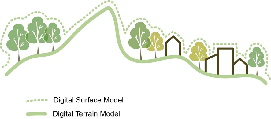
As this study is assessing the visibility of some of the indicators, the analysis required a Digital Terrain Models (DTM) to simulate the topology of the Earth. Ordnance Survey (OS) Terrain 50 and the National LIDAR Programme were used to develop this surface. They are both DTMs which only take into account the bare surface of the Earth and do not include features such as trees and buildings that rise above the ground.

Given the importance of buildings and trees in constraining visibility, these DTMs were converted into Digital Surface Models (DSMs) by modelling in the trees and buildings using data from OS MasterMap and the National Forest Inventory data from the Forestry Commission. Figure ‎2.3 illustrates the difference between a DTM and a DSM.

Figure 2.3: Digital Terrain Models and Digital Surface Models

As the All South and Vale and Urban components of this study are assessed separately and at different scales, the datasets used to generate the surfaces for each were different.

 

All South and Vale

For the All South and Vale surface, OS Terrain 50 (OST50) data was used. This data has a resolution (pixel size) of 50 metres. Given this resolution, it was likely that many pixels would only be partially covered by buildings or trees, and so raising their elevation value to the height of that surface feature would vastly overstate the visibility obstruction. However, only raising the pixel value where the whole pixel was covered in surface features would do the opposite. In order to balance these factors, a pixel value was raised if more than 20% of its area was covered by buildings or trees.

The building data used was OS MasterMap, and the woodland data was from the National Forest Inventory. Notional values needed to be applied to augment the surface model. The values were presented to stakeholders during the workshop. The values used to raise the bare ground model are as shown in Table ‎2-1.

Table ‎2-1: Height of objects added to the elevation model

Surface feature	Elevation increases (metres)
Building	8
Assumed woodland	10
Broadleaved woodland	10
Conifer woodland	15
Coppice	3
Coppice with standards	3
Low density woodland	8
Mixed mainly broadleaved woodland	12
Mixed mainly conifer woodland	12
Shrub	3
Young trees	5

Where multiple features met the 20% coverage criteria, the highest value was taken. Pixels that intersected with roads, paths, railways, rivers and waterbodies were removed so as not to overstate their visibility.

 

Urban

The process for the generation of the Urban surface was the same as for All South and Vale, except using the National LIDAR Programme DTM 1 metre resolution resampled to 10 metres as the base instead of OST50. The National LIDAR Programme DTM is very high resolution, providing detailed surface information. However processing the visibility analysis with this resolution of data would be impractical, so the National LIDAR Programme DTM was resampled to 10m pixels. This involved reducing the resolution of the data and taking an average of each original pixel that falls within the 10m cell (or pixel).

The Urban surface was only generated out to 6km from the selected urban areas (Figure ‎2.2). The reasons for this are covered under the Data processing heading later in this section.

For consistency in approach, the 20% overlap method was also used for the generation of this surface. In this case, the building data was OS MasterMap, and instead of giving each building an assumed height of 8 metres, each building was given an individual height from the OS MasterMap Building Height Attribute (BHA) data. Woodland data was from the National Forest Inventory, using the same assumed heights as for the All South and Vale surface (Table ‎2-1). In the urban areas themselves the woodland data was removed to avoid double counting when it came to the visibility analysis.

Back to top

Data processing

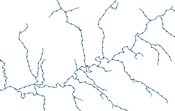
Visibility analysis is calculated from specific locations to all pixels within the surface dataset. These specific locations are represented in GIS as ‘points’ – discrete pieces of data with x and y coordinates, but no area or length. Because of this, any datasets stored as polygons needed to be converted so that they were represented as points. In all instances, this involved generating a grid of points at equal intervals covering the study area. Those points that intersected the polygons were then used as the basis of the visibility analysis. For smaller features that may be missed by the grid, the outlines of the polygons were converted into points, with points at a set distance around the perimeter.

Visibility analysis can be run from lines, but for consistency these were converted into points for the analysis as shown in Figure ‎2.4.

Figure 2.4: Approach to generating point layers from features

The specific details of the method and grid density for each indicator are detailed in the Positive indicators details (Chapter 3) and Negative indicators details (Chapter 4) sections.

For all visibility analysis, the maximum processing distance was set to 6 km from the source points. This is in accordance with the CPRE study for England, which itself drew the conclusions from Benson et al (2002) [See reference [i]]. The CPRE methodology utilised a distance of 6 km to model the theoretical limit of visibility. Earth curvature was taken into account in the visibility analysis. Therefore, scores greater than 0 are only assigned where the model indicates that a feature is theoretically visible when both earth curvature and elevation are accounted for, with the elevation including buildings and vegetation as detailed in the Generation of analysis surfaces section above.

Indicators relating to hearing either natural or detracting sounds have been assessed based on distance from the source of the sound. Decibel (dB) is the measurement unit used for indicating the intensity of a sound as perceived by the human ear. The more intense a sound is, the higher up it will be on the decibel scale.

Extensive literature review and stakeholder engagement was carried out by LUC as part of the Tranquillity and Place Sound Environment project [See reference [ii]] in Wales to establish buffers for sound indicators in tranquillity assessments. It was found that sound is expected to drop by 6 dB each time the distance from the source is doubled (Collman (2015)) [See reference [iii]]. For example, a sound that is 60 dB at 5 metres from the source would decrease as per Table ‎2-2. For reference, an increase of 10 dB corresponds to a tenfold (ten times) increase in sound intensity and is perceived as twice as loud.

Table ‎2-2: Sound decreases when distance increases

Distance (m)	5	10	20	40	80	160	320	640
Sound (dB)	60	54	48	42	36	30	24	18

The analysis expects that there would be an ambient background noise level of 30 dB in rural areas (Mehta et al. (1999)) [See reference [iv]]. Sounds below that level would just contribute to that background noise rather than being distinct sounds. As such the analysis only measures out to a distance where sounds would be above 30 dB. For instance, in the example above, the analysis would only extend out to 160m away from the source of the sound.

The same process was applied to the Urban analysis where the ambient sound is expected to be higher than in rural areas and is likely to have variations in background level. King et al. (2012) suggest that in urban areas, once a sound is below 40dB it becomes indistinguishable from the general sounds associated with an urban area.

[i] Benson, John F, Jackson, Susan P and Scott, Karen E University of Newcastle. (2002). Visual Assessment of Windfarms: Best Practice, Scottish Natural Heritage Commissioned Report F01AA303A, Edinburgh.

[ii] Green C, Manson D, Chamberlain K. (2022). NRW Report No: 569, 185 pp, NRW. Available at: https://storymaps.arcgis.com/stories/865c1876d9f64280a3dfc6e2769a46a5

[iii]Collman, R. (2015) Distance Attenuation https://www.acoustical.co.uk/distance-attenuation/how-sound-reduces-with-distance-from-a-point-source/

[iv] Mehta, M., Johnson, J., and Rocafort, J. (1999) Architectural Acoustics: Principle and Design. Merrill Prentice Hall. Upper Saddle River, NJ.

 

Back to top

Scoring

Once all the visibility analysis was complete, buffers were generated around the source datasets representing the features from which the visibility was being calculated. For most indicators in All South and Vale these were at the following distances:

• 500 metres
• 1 kilometre
• 2 kilometres
• 5 kilometres
• 6 kilometres

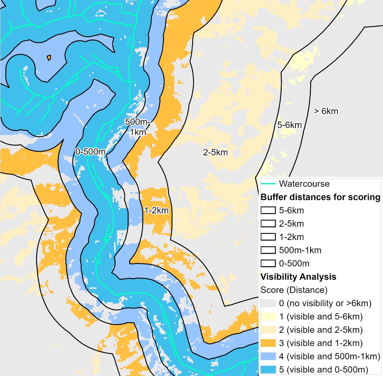
To represent features that are closer having more visual impact than features that are further away, these buffers were then combined with the results of the visibility analysis to work out if a pixel is both within a certain distance, and visible. The pixels were then scored based on these factors. The scoring varies for each indicator but has a maximum value of 5 (highest contribution to tranquillity for positive indicators, lowest contribution to tranquillity for negative indicators) and a minimum of 0 (no contribution to tranquillity). An example of the scoring can be found in Table ‎2-3: This illustrates the scoring approach for a feature that contributes to tranquillity using the seeing rivers indicator as an example in Figure ‎2.5.

Figure 2.5: Contributing buffer distance and scores visibility analysis

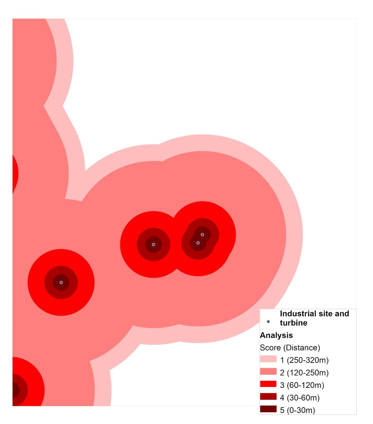
Sounds that detract from tranquillity were given a higher detracting score closer to the source. When the distance increases from the source, the sound level decreases, therefore lower scores were given for further distances. This is shown visually for sounds that detract from tranquillity using the hearing non-natural sound indicator as an example in Figure ‎2.6.

Figure 2.6: Detracting buffer distances and scores

Back to top

Combination of indicators

Once all of the positive and negative indicators were scored, they were combined together to give a total positive and negative score for each pixel.

• Overall positive score All South and Vale – a high score means the pixel is more tranquil
• Overall negative score All South and Vale – a high score means the pixel is less tranquil

The All South and Vale and Urban analyses are processed and combined separately.

Back to top

Producing the tranquility map

The analysis results represent the spatial distribution of relative tranquillity across South Oxfordshire and Vale of White Horse District Councils. The relative tranquillity is calculated as the difference between the overall positive score and the overall negative score.

Chapter 2 and Chapter 3 provide specific details on the data sources, method and results for each of the indicators.